Here, we train our first Neural Network to classify handwritten digits.
A Multi-class Classification Example
Loading MNIST Dataset
The MNIST (Modified National Institute of Standards and Technology) is a dataset of images of handwritten digits 0 to 9. More information about the dataset can be seen on this website.
We load the dataset which is available via the keras package. Then we store and training and test images and labels separately.
Code
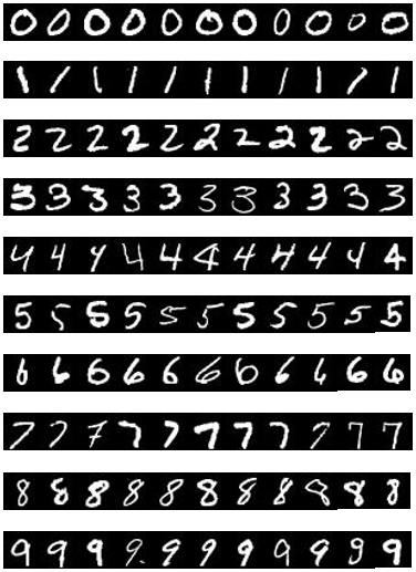
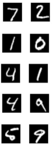
library(keras)mnist =dataset_mnist()train_images <- mnist$train$xtrain_labels <- mnist$train$ytest_images <- mnist$test$xtest_labels <- mnist$test$y# code to plot 1st 10 test images (useful at end)par(mfrow=c(5,2))for(i in1:10){ plot(as.raster(test_images[i,,], max=255)) }par(mfrow=c(1,1))
Glimpse into our Data
Basic Understanding
Before we divide into to creating our model using tensorflow, let’s understand few concepts like tensors and tensor operations.
A Tensor is a generalisation of vectors and matrices to an arbitrary number of dimensions/axis.
Tensor
R object
0 dimensional tensor
scalar
1 dimensional tensor
vector
2 dimensional tensor
matrix
3d or higher tensor
array
A ‘Scalar’ is a tensor that contains only 1 number. An R vector of length 1 is a scalar. ‘Vectors’ are one-dimensional tensor e.g. c(12,3,4,10,5) has 5 elements but 1 dimension
Code
x =c(12,3,6,14,10) dim(as.array(x)) # dimension = 5
A ‘Matrix’ is a two-dimensional tensor. For example, A matrix(rep(0,35),3,5) which returns a null-matrix of order 3x5. Thus, the 2 dimensions are ‘rows’ and ‘columns’. We say that the shape of a 2d tensor is (samples, features).
Code
x =matrix(rep(0,35),3,5) dim(x) # dimension = 3,5
An ‘Array’ is a three-dimensional tensor. The shape of 3d tensor is (samples, timesteps, features) e.g. a Time Series or Sequence Data like of stock price can be represented by a 3d tensor of shape (250, 390, 3) where 250 = number of trading days, 390 = minutes per trading day, 3 = current price, highest price, lowest price in past minute. Let’s look at an e.g. of sequence
Code
x =array(rep(0,2*3*2),dim=c(2,3,2)) dim(x) # dimension = 2,3,2
The shape of a ‘4d tensor’ is (samples, height, width, channels) e.g. images like (128, 256, 256, 1) where 128 is the number of gray-scale images of size 256x256, channels = 1 indicates gray-scale whereas channels = 3 indicates Red-Green-Blue i.e. coloured-images.
The shape of ‘5d tensor’ is (samples, frames, height, width, channels) e.g. a video file.
3 Key attributes
No. of Axes - for example a 3D tensor has 3 axes and a matrix has 2 axes i.e. rows and columns.
Code
length(dim(train_images)) # no. of axes of tensor = 3
Shape - an integer vector that describes how many dimensions the tensor has along each axis. For eg. the previous matrix eg has shape (3,5)
Code
dim(train_images) # shape = (60000,28,28)
Data Type - the type of data contained in the tensor, for e.g. a tensor’s type could be integer or double. There could also be a character tensor.
Code
typeof(train_images) # data type = integer
Tensor Operations
Slice Operation : involves selecting specific elements in a tensor.
Code
myslice = train_images[10:99,,] # selecting digits 10 to 99
We can slice a tensor into batches.
Code
batch = train_images[1:128,,]
dim(batch)
When considering such a batch tensor, the first axis is called the or batch axis/ batch dimension.
Tensor Dot Operation : involves combining entries in input tensors doing using %*% and element wise product is done using * e.g. we have x of shape (a,b) and y of shape (b,c) then their dot product z has shape (a,c)
Tensor Re-shaping : means rearranging its rows and columns to match a specific shape.
Code
x =matrix(c(0,1,2,3,4,5),3,2,byrow = T) # 2 rows and 3 columns x =array_reshape(x, dim=c(2,3)) # 3 rows and 2 columns x =array_reshape(x, dim=c(6,1)) # 6 rows and 1 column
Data Preparation
Currently our we have 60,000 images, which are of the dimension 28 by 28. To feed them to a neural network, we need to convert them into a long vector of numbers. We do this by using array_reshape() command. So from 28 by 28 we end up with 784 as the dimension of all the 60,000 images. Next, we divide these numbers by 255 to ensure that the range of all numbers is [0,1].
At last, we need to convert the labels into categories, which can be easily done by using the to_categorical() command.
keras_model_sequential() tells R to stack the following layers linearly; one after another.
This network has two layers. They are called dense layers because every neuron in the layer is connected to the neurons in the previous layer i.e. fully connected. So, the 2nd layer’s neurons receive input from all the neurons in previous layers.
The 1st layer_dense has 512 neurons/units. Our input image is of the dimension 28 by 28 . So, the layer receives inputs of shape 28*28 because we convert the image into a long vector of numbers. Every neuron is associated with a ReLU Activation function.
ReLU stands for Rectified Linear Unit. Basically, ReLU(z) = max(0 , z). It is a piece-wise linear function which returns zero when dealing with negative values and returns the identity function in the positive side.
The 2nd layer is the output layer with 10 neurons. Using softmax activation allows us to receive probabilities of a particular image belonging to 0-9 category.
Compile
After creating the network structure, we need to compile the network. This step has 3 elements :
Loss Function - This allows the network to measure performance and steer itself in the right direction. The idea is to minimize the value of the loss function to maximise accuracy metrics.
Optimizer - This is the mechanism by which network updates it’s parameters while minimizing the loss function.
Metrics - These are figures indicating the performance of the model like Accuracy, MAPE, MSE.
Here, we use the loss function categorical_crossentropy because we are dealing with output in multiple categories from digits 0 to 9. The optimizer rmsprop provides R with information about how we need to minimize the loss function.
Choosing The Right Loss Function
‘Cross-entropy’ measures the distance between probability distributions or, in this case, between ground-truth distribution and our predictions. Thus, it is usually the best choice when dealing with models that output probabilities.
‘Binary Cross-entropy’ is used when we are dealing with binary classification problems. Whereas, when dealing with problem where the output has more than 2 classes, we use ’Categorical Cross-entropy’.
Here, is a small guide on choice of loss function based on last layer of the model :
Problem Type
Last Layer Activation
Loss Function
Binary Classification
Sigmoid
Binary crossentropy
Multi-class single-label classification
Softmax
Categorical crossentropy
Multi-class multi-label classification
Sigmoid
Binary crossentropy
Regression to arbitrary value
None
Mean Squared Error (MSE)
Regression to value {0,1}
Sigmoid
MSE or Binary crossentropy
Training
Now we are ready to train our model !
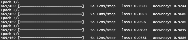
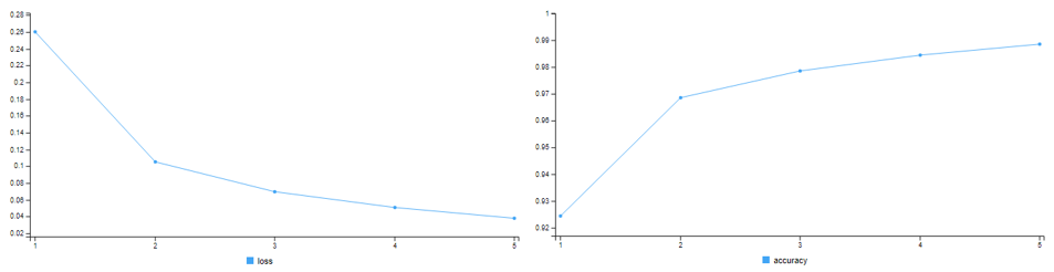
The network will go over the training data in mini-batches of 128 samples, 5 times over at each iteration, the network computes the gradient of the weights with regard to the loss on the batch, and update the weights accordingly.
With every iteration, the network was able to minimize the error and improve upon it’s accuracy. At the end of 5 tries, the network achieves a classification-accuracy of 98.86% on the training images where we had provided labels.
Evaluation & Prediction
Let’s see how our model performs on test images where we have no provided the labels. This will be the true test of the network’s capabilities !